Homework 9 - Alligators
Ammar Plumber, Elaina Lin, Kim Nguyen, Meghan Aines, Ryan Karbowicz
4/13/2021
I. Introduction
Social media has evolved and affected our lives in many aspects. In this assignment, we aim to have a closer look at two of the most popular social media platforms: Tiktok and Facebook. These platforms are in a similar industry but with very different target audiences, thus the two brands and their audiences could differ in their communication styles and language. Understanding the language used in these platforms may lead to their business implications and directions.
Our research question examines whether there are differences in sentiments of tweet communications that mention Tiktok and Facebook accounts.
II. Methodology
Our method of sentiments analysis is text mining with R.
First, after getting tweets from twitter, we use basic tools of data exploration to transform, visualize, and examine different features of the datasets, such as source, time, length, and content (e.g, link and picture) of the tweets. We produce bar charts to visualize the most popular words used by each twitter account, as well as the most popular sentiments associated with tweets that each account produces. A wordcloud also helps paint a clearer picture of each company’s most commonly used words.
Second, we transform the datasets into tidy text format for sentiment analysis. The two main lexicons that we use are nrc and affin.
Finally, we run 4 different models to predict if a tweet was posted by either Facebook or Tiktok. The inputs of these models are the length of the tweet, as well as sentiment (which includes anger, anticipation, disgust, negative, postive, trust, joy, surprise, fear and sadness).
The first model is a Simple Decision Tree, the second model is a Bagging Model, the third model is a Random Forest and the fourth model is a Gradient Boosting Model.
Our results include a sum of squares analysis on the test set of data to determine which models have the smallest differences between the predicted tweeter and actual tweeter. We also include confusion matrices on the test set of data to analyze the prediction accuracy of the 4 models.
#Loading packages.
library(rtweet)
library(tidyverse)
library(lubridate)
library(scales)
library(tidytext)
library(wordcloud)
library(textdata)

library(caret)       # for general model fitting
library(rpart)       # for fitting decision trees
library(rpart.plot)
library(ipred)       # for fitting bagged decision trees
library(ranger)
library(gbm)
library(vip)
library(kableExtra)
#Getting tweets
# Run these two lines to get the tweets
# and then save them as a csv for future use
# tiktok <- get_timeline("tiktok_us", n=3200)
# tiktok %>% write_as_csv('tiktok.csv')
#
# facebook <- get_timeline("Facebook", n=3200)
# facebook %>% write_as_csv("facebook.csv")
tiktok <-
read_csv('tiktok.csv') %>%
select(status_id, source, text, created_at)
facebook <-
read_csv('facebook.csv') %>%
select(status_id, source, text, created_at)
nrc <- read_rds("nrc.rds")
facebook %>% head()## # A tibble: 6 x 4
## status_id source text created_at
## <chr> <chr> <chr> <dttm>
## 1 x1382020080343~ Twitter W~ "Ramadan Mubarak <U+0001F319>\r\n \r\nThis #Mo~ 2021-04-13 17:17:18
## 2 x1381734429018~ Khoros CX "@MeenalK1 Hi Meenal. Do you have the referenc~ 2021-04-12 22:22:13
## 3 x1381733382632~ Khoros CX "@Afrojalipro Thanks for updating us, Afroj! W~ 2021-04-12 22:18:04
## 4 x1381732668388~ Khoros CX "@CallandManning Hi Calland. If you do not hav~ 2021-04-12 22:15:14
## 5 x1381711376876~ Khoros CX "@BHARTINANDAN4 Hello! Please visit this Help ~ 2021-04-12 20:50:37
## 6 x1381710548476~ Khoros CX "@weathermatt22 Hi Matt. Please visit our Help~ 2021-04-12 20:47:20facebook %>%
count(source, hour = hour(with_tz(created_at, "EST"))) %>%
mutate(percent = n/sum(n)) %>%
ggplot(aes(x = hour, y = percent, color = source)) +
labs(x = "Hour of day (EST)", y = "% of tweets", color = "") +
scale_y_continuous(labels = percent_format()) +
geom_line() +
ggtitle('Facebook Source Breakdown by Hour')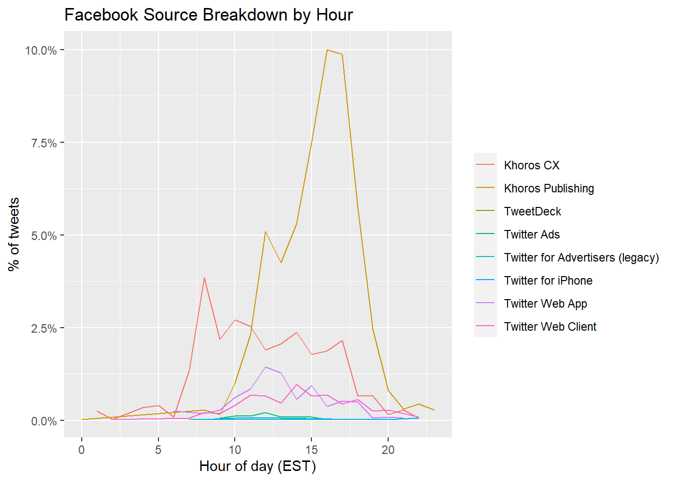
tiktok %>%
count(source, hour = hour(with_tz(created_at, "EST"))) %>%
mutate(percent = n/sum(n)) %>%
ggplot(aes(x = hour, y = percent, color = source)) +
labs(x = "Hour of day (EST)", y = "% of tweets", color = "") +
scale_y_continuous(labels = percent_format()) +
geom_line() +
ggtitle('Tiktok Source Breakdown by Hour')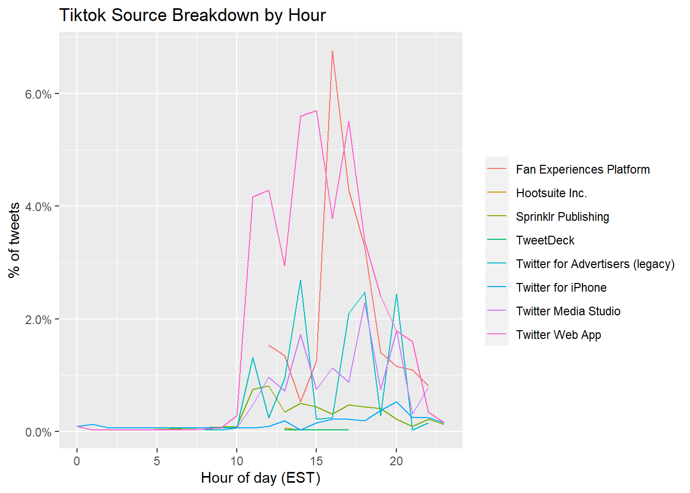 These above figures indicate Tiktok/Facebook breakdown by hour. Across sources, the “busiest” time on both platforms are from 12:00 to 20:00. While Khoros Publishing has the most tweets about Facebook with its peak around 16:00, Twitter Web App and Fan Experiences (peaks around 16:00) are the main source of tweets about Tiktok.
fb_wordcounts <-
  facebook %>%
  mutate(tweetLength = str_length(text)) %>%
  filter(tweetLength < 500)

tiktok_wordcounts <-
  tiktok %>%
  mutate(tweetLength = str_length(text)) %>%
  filter(tweetLength < 500)

writeLines(c(paste0("Facebook Mean Tweet Length: ",
                  mean(fb_wordcounts$tweetLength)),
           paste0("TikTok Mean Tweet Length: ",
                  mean(tiktok_wordcounts$tweetLength))))
## Facebook Mean Tweet Length: 163.370231394622
## TikTok Mean Tweet Length: 112.916405760801hist(tiktok_wordcounts$tweetLength)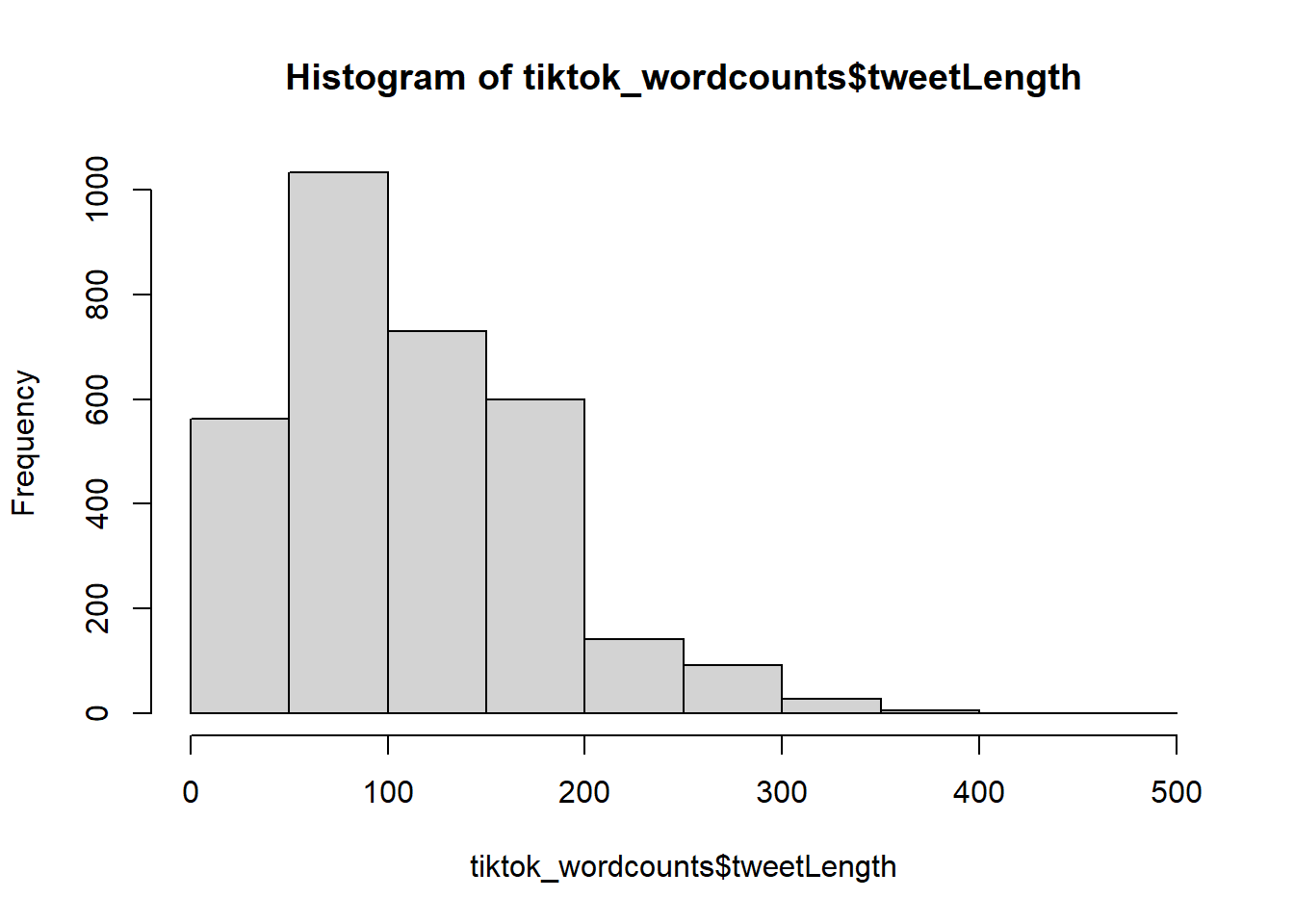
hist(fb_wordcounts$tweetLength)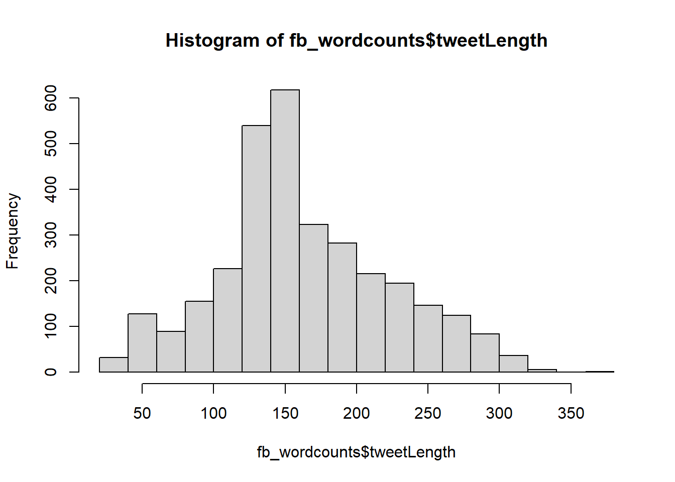
In terms of tweet length, a typical tweet related to Tiktok has from 50 to 100 words. There are less tweets that has more than 100 words. A typical tweet related to Facebook has around 150 words.
fb_picture_counts <-
  facebook %>%
  filter(!str_detect(text, '^"')) %>%
  count(picture = ifelse(str_detect(text, "t.co"),
                         "Picture/link", "No picture/link"))

tiktok_picture_counts <-
  tiktok %>%
  filter(!str_detect(text, '^"')) %>%
  count(picture = ifelse(str_detect(text, "t.co"),
                         "Picture/link", "No picture/link"))

barplot(fb_picture_counts$n,
        names.arg=c("No picture/link", "Picture/link"),
        main = "Facebook # of Tweets with and without pics/link")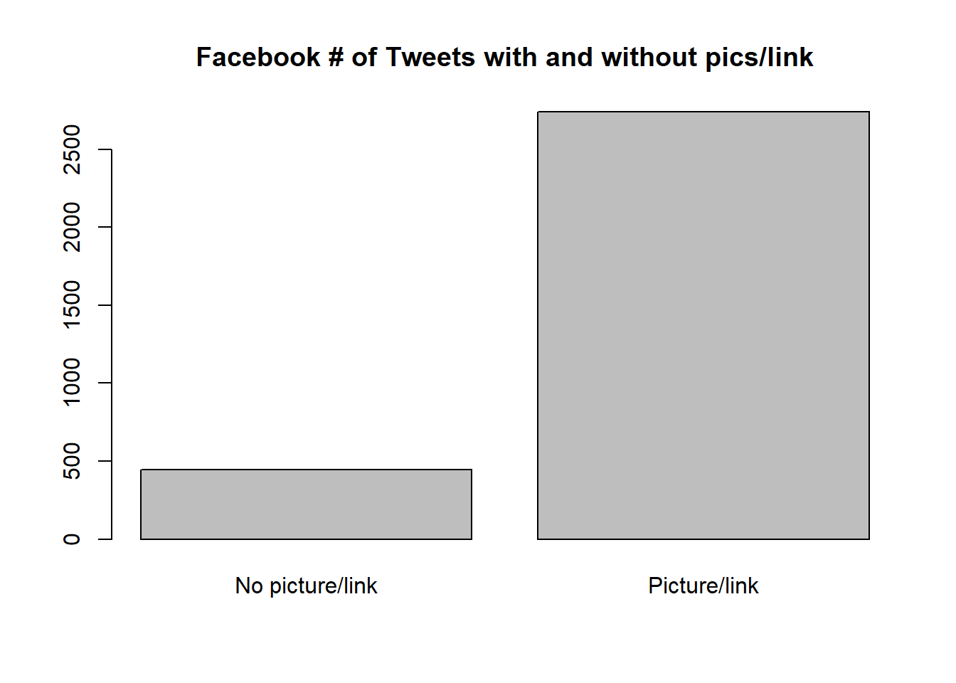
barplot(tiktok_picture_counts$n,
        names.arg=c("No picture/link", "Picture/link"),
        main = "Tiktok # of Tweets with and without pics/link")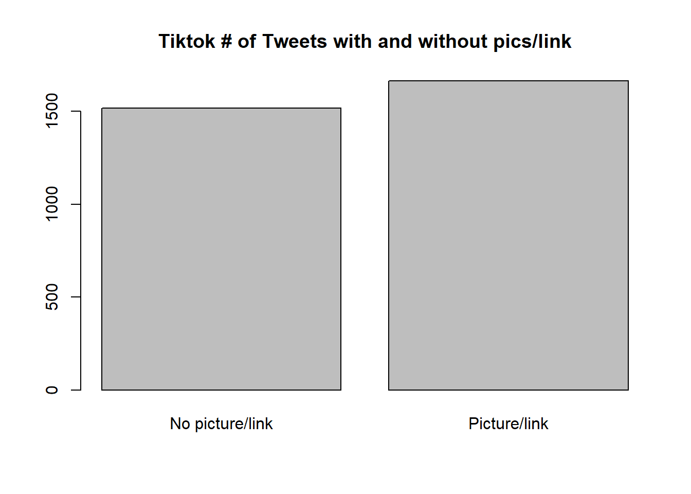
Facebook tweets that contains pictures or links are more common than ones that have no pictures or links. There are no remarakble differences between tweets that contain picture/link and ones that don’t contains picture/link from Tiktok.
reg <- "([^A-Za-z\\d#@']|'(?![A-Za-z\\d#@]))"
# Unnest the text strings into a data frame of words
fb_words <-
facebook %>%
filter(!str_detect(text, '^"')) %>%
mutate(text = str_replace_all(text,
"https://t.co/[A-Za-z\\d]+|&",
"")) %>%
unnest_tokens(word, text,
token = "regex",
pattern = reg) %>%
filter(!word %in% stop_words$word,
str_detect(word, "[a-z]"))
tiktok_words <-
tiktok %>%
filter(!str_detect(text, '^"')) %>%
mutate(text = str_replace_all(text,
"https://t.co/[A-Za-z\\d]+|&",
"")) %>%
unnest_tokens(word, text,
token = "regex",
pattern = reg) %>%
filter(!word %in% stop_words$word,
str_detect(word, "[a-z]"))
# Inspect the first six rows of tweet_words
head(fb_words)## # A tibble: 6 x 4
## status_id source created_at word
## <chr> <chr> <dttm> <chr>
## 1 x1382020080343470082 Twitter Web App 2021-04-13 17:17:18 ramadan
## 2 x1382020080343470082 Twitter Web App 2021-04-13 17:17:18 mubarak
## 3 x1382020080343470082 Twitter Web App 2021-04-13 17:17:18 0001f319
## 4 x1382020080343470082 Twitter Web App 2021-04-13 17:17:18 #monthofgood
## 5 x1382020080343470082 Twitter Web App 2021-04-13 17:17:18 check
## 6 x1382020080343470082 Twitter Web App 2021-04-13 17:17:18 kindnessfb_words %>%
count(word, sort = TRUE) %>%
head(20) %>%
mutate(word = reorder(word, n)) %>%
ggplot(aes(x = word, y = n)) +
geom_bar(stat = "identity") +
ylab("Occurrences") +
coord_flip()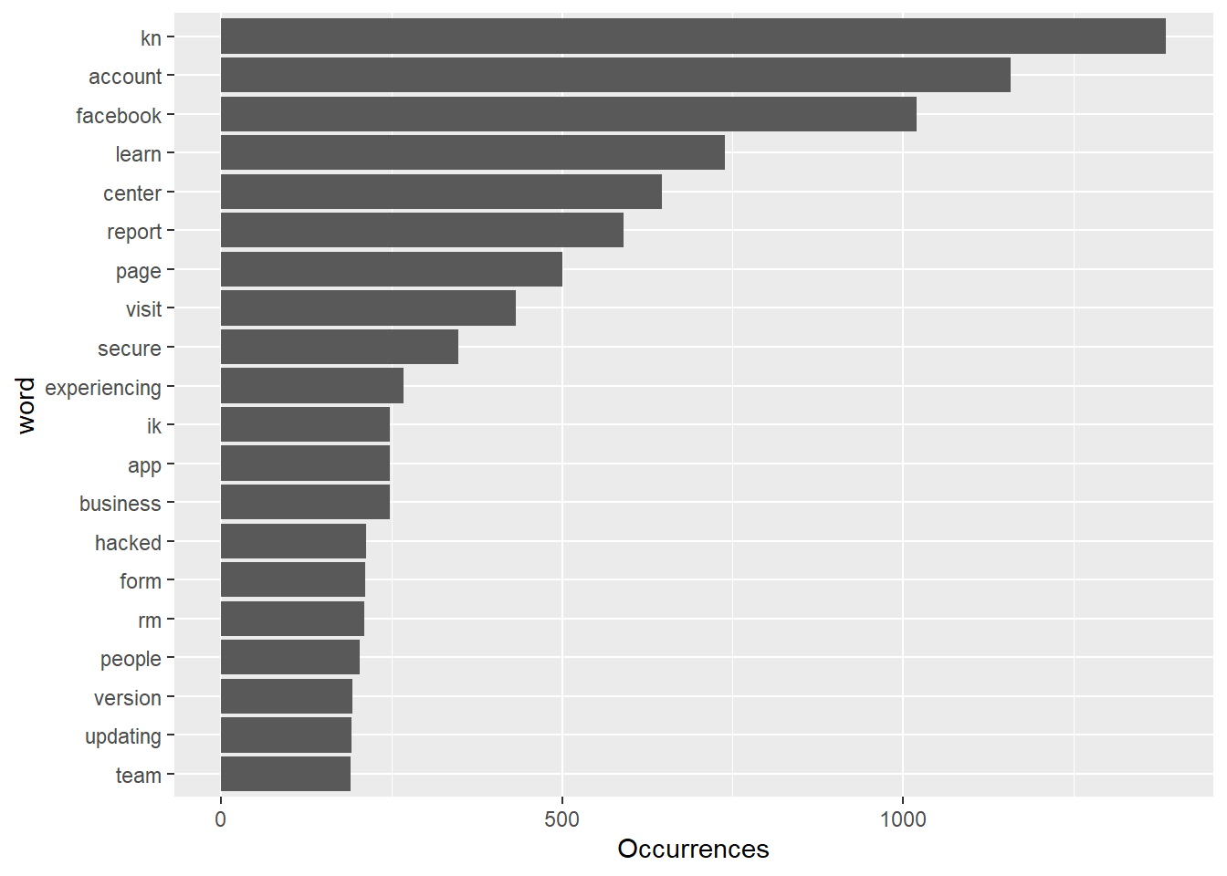
tiktok_words %>%
  count(word, sort = TRUE) %>%
  head(20) %>%
  mutate(word = reorder(word, n)) %>%
  ggplot(aes(x = word, y = n)) +
  geom_bar(stat = "identity") +
  ylab("Occurrences") +
  coord_flip()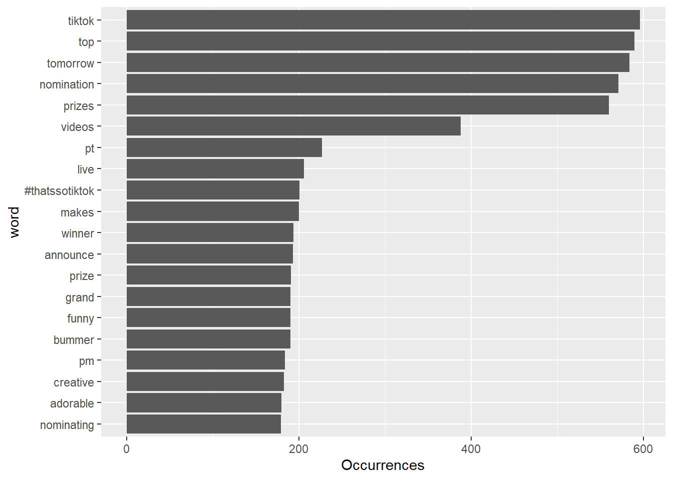
fb_sentiment <-
 inner_join(fb_words, nrc, by = "word") %>%
            group_by(sentiment)

tiktok_sentiment <-
 inner_join(tiktok_words, nrc, by = "word") %>%
            group_by(sentiment)

fb_words %>% head()
## # A tibble: 6 x 4
## status_id source created_at word
## <chr> <chr> <dttm> <chr>
## 1 x1382020080343470082 Twitter Web App 2021-04-13 17:17:18 ramadan
## 2 x1382020080343470082 Twitter Web App 2021-04-13 17:17:18 mubarak
## 3 x1382020080343470082 Twitter Web App 2021-04-13 17:17:18 0001f319
## 4 x1382020080343470082 Twitter Web App 2021-04-13 17:17:18 #monthofgood
## 5 x1382020080343470082 Twitter Web App 2021-04-13 17:17:18 check
## 6 x1382020080343470082 Twitter Web App 2021-04-13 17:17:18 kindnessHere we compare the sentiment between Facebook and TikTok. It looks like discussions surrounding Facebook uses more trust words while topics about TikTok uses more words that reflect anticipation.
fb_sentiment_analysis <- fb_sentiment %>%
  count(word, sentiment) %>%
  group_by(sentiment)

fb_sentiment_analysis %>%
  top_n(15) %>%
  ggplot(aes(x = sentiment, y = n )) +
  geom_bar(stat = "identity") +
  coord_flip() +
  ylab("Frequency") +
  xlab("Sentiment") +
  labs(title="Facebook Sentiment")
## Selecting by n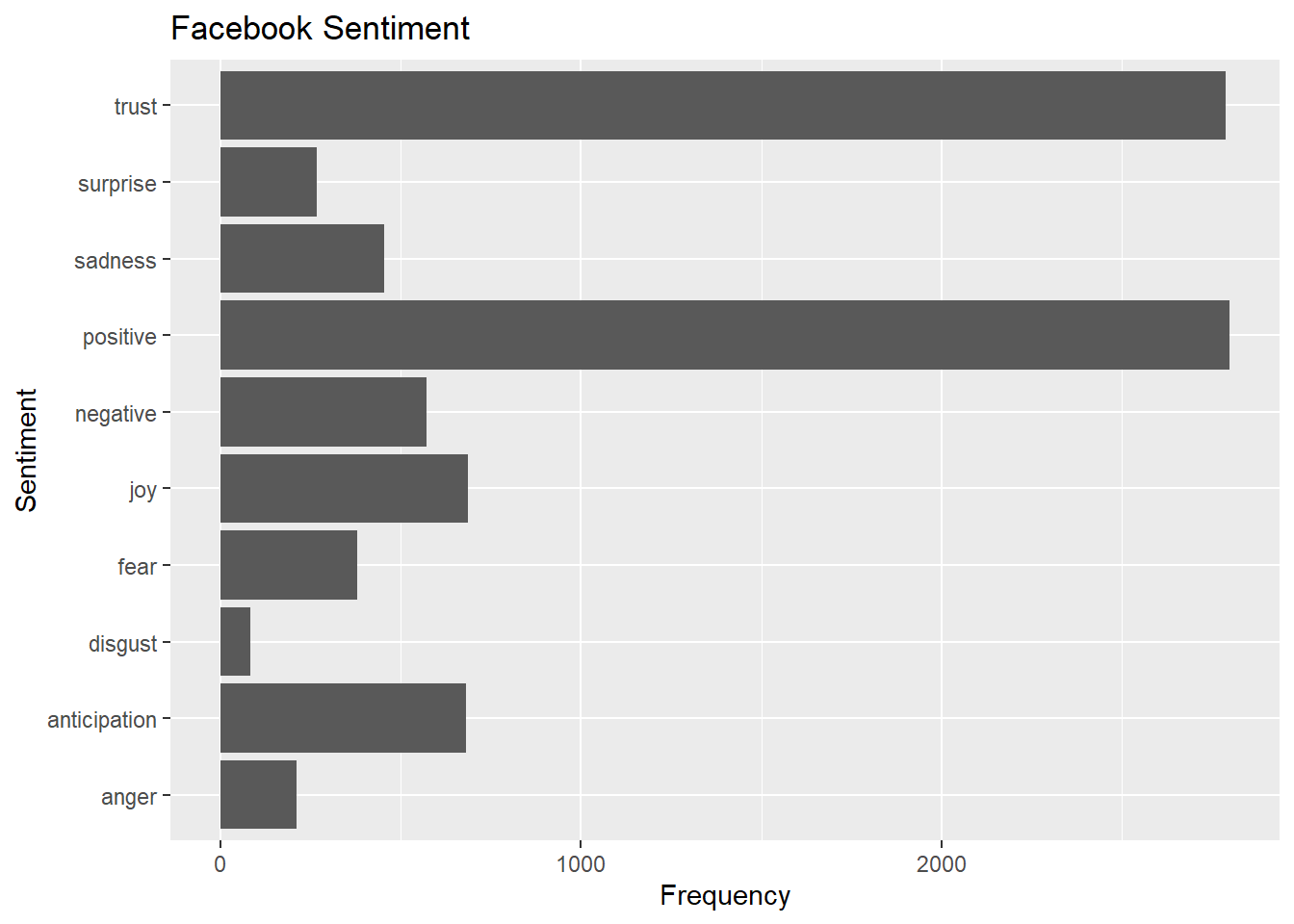
tiktok_sentiment_analysis <- tiktok_sentiment %>%
  count(word, sentiment) %>%
  group_by(sentiment)

tiktok_sentiment_analysis %>%
  top_n(15) %>%
  ggplot(aes(x = sentiment, y = n )) +
  geom_bar(stat = "identity") +
  coord_flip() +
  ylab("Frequency") +
  xlab("Sentiment") +
  labs(title="TikTok Sentiment")
## Selecting by n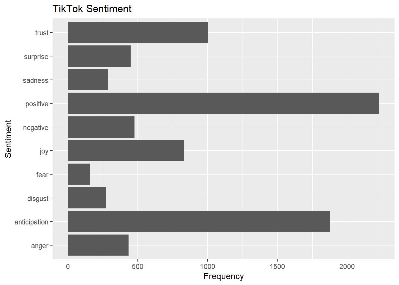
fb_sentiment_analysis %>% filter(!sentiment %in% c("positive", "negative")) %>%
  mutate(sentiment = reorder(sentiment, -n),
         word = reorder(word, -n)) %>% top_n(10) -> fb_sentiment_analysis2
## Selecting by nggplot(fb_sentiment_analysis2, aes(x=word, y=n, fill = n)) +
facet_wrap(~ sentiment, scales = "free")+
geom_bar(stat ="identity") +
theme(axis.text.x = element_text(angle = 90, hjust = 1)) +
labs(y="count", title="Facebook Sentiment")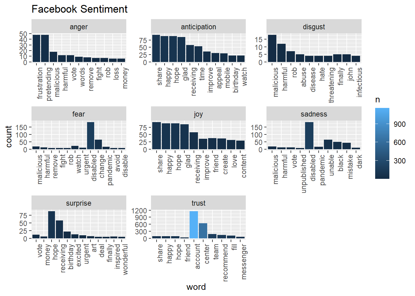
tiktok_sentiment_analysis %>% filter(!sentiment %in% c("positive", "negative")) %>%
  mutate(sentiment = reorder(sentiment, -n),
         word = reorder(word, -n)) %>% top_n(10) -> tiktok_sentiment_analysis2
## Selecting by nggplot(tiktok_sentiment_analysis2, aes(x=word, y=n, fill = n)) +
facet_wrap(~ sentiment, scales = "free")+
geom_bar(stat ="identity") +
theme(axis.text.x = element_text(angle = 90, hjust = 1)) +
labs(y="count", title="Tik Tok Sentiment")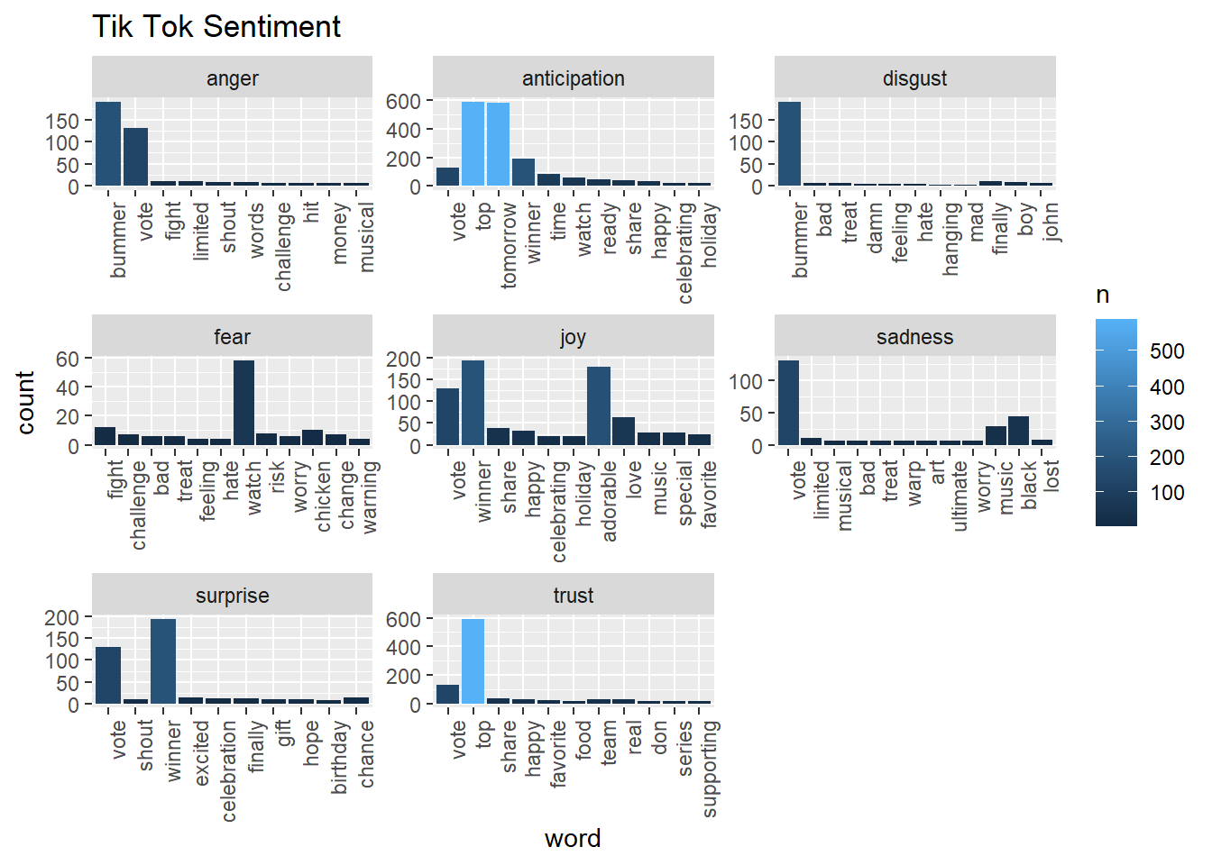
We also want to visualize common words on Facebook and Tiktok by Wordcloud. The visual depiction indicates to us that “learn”, “center” and “report” are common words, with more secondary common words such as “secure” page“, and”visit" for Facebook account engagement. This could be that Facebook users tweet about account issues. Whereas, TikTok has “top”, “tomorrow”, and “prizes” as common words, and more secondary common words such as “winner,”nominating“, and”grand", indicating that the social media platform likes to promote competitions or giveaways, which makes sense given their younger demographics might enjoy these types of rewards and games.
facebook_cloud <- fb_words  %>% count(word) %>% arrange(-n)
wordcloud(facebook_cloud$word, facebook_cloud$n, max.words = 200, colors = c("#00B2FF", "red", "#FF0099", "#6600CC", "green", "orange", "blue", "brown"))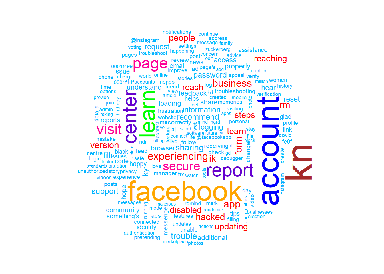
tiktok_cloud <- tiktok_words  %>% count(word) %>% arrange(-n)
wordcloud(tiktok_cloud$word, tiktok_cloud$n, max.words = 200, colors = c("#00B2FF", "red", "#FF0099", "#6600CC", "green", "orange", "blue", "brown"))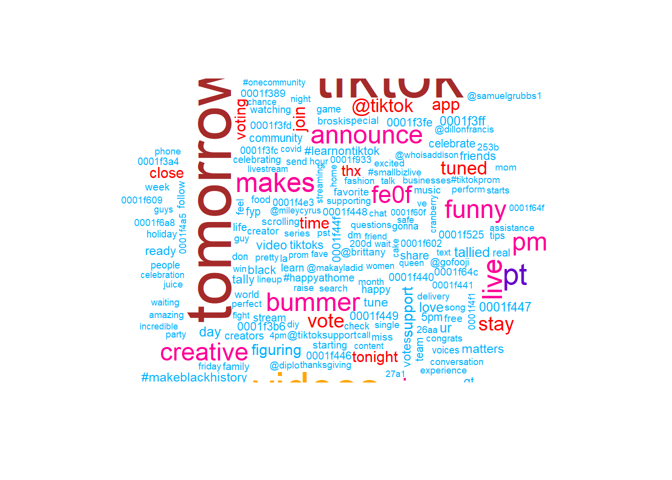
Next, we examine texts on Facebook and Tiktok to see their positive-negative score by using the AFINN sentiment lexicon, a list of English terms manually rated for valence with an integer between -5 (negative) and +5 (positive) by Finn Årup Nielsen between 2009 and 2011.
We use this lexicon to compute mean positivity scores for all words tweeted by each user.
# run this to get afinn lexicon and save it as a csv
# get_sentiments ("afinn") -> afinn
#
#afinn %>% write_as_csv("afinn.csv")
afinn <- read_csv('afinn.csv')
fb_afinn <-
 inner_join(fb_words,
            afinn,
            by = "word")
tiktok_afinn <-
 inner_join(tiktok_words,
            afinn,
            by = "word")
fb_mean_afinn <-
  fb_afinn %>%
  summarise(mean_fb_afinn = mean(value))
tiktok_mean_afinn <-
  tiktok_afinn %>%
  summarise(mean_tt_afinn = mean(value))
cat(paste0("Average AFINN scores for all words by user\n",
           "\nFacebook: ", round(fb_mean_afinn, 3),
           "\nTikTok: ", round(tiktok_mean_afinn, 3)))
## Average AFINN scores for all words by user
##
## Facebook: 0.785
## TikTok: 1.704Facebook’s mean AFINN value is 0.79 while TikTok’s mean AFINN value is 1.704. In general, words tweeted by Tiktok are more positive than those tweeted by Facebook.
Training Predictive Models
Here, using the text of a tweet, we attempt to predict the user who tweeted it.
The features we extracted are tweet length, the presence of a picture/link, number of words for each sentiment, and mean AFINN score per tweet.
TikTok is encoded as 1, and Facebook is encoded as 0.
First, we produce a simple decision tree.
fb_piclinks <-
  facebook %>%
  filter(!str_detect(text, '^"')) %>%
  mutate(picture_link = ifelse(str_detect(text, "t.co"),
                         1, 0)) %>%
  select(1,5)
tiktok_piclinks <-
  tiktok %>%
  filter(!str_detect(text, '^"')) %>%
  mutate(picture_link = ifelse(str_detect(text, "t.co"),
                         1, 0)) %>%
  select(1,5)
fb_tweet_afinn <-
  fb_afinn %>%
  group_by(status_id) %>%
  summarize(afinn = mean(value))
## `summarise()` ungrouping output (override with `.groups` argument)tiktok_tweet_afinn <-
tiktok_afinn %>%
group_by(status_id) %>%
summarize(afinn = mean(value))## `summarise()` ungrouping output (override with `.groups` argument)fb_sentiment_counts <-
fb_sentiment %>%
group_by(status_id) %>%
count(sentiment) %>%
pivot_wider(id_cols = status_id,
names_from = sentiment,
values_from = n,
values_fill = 0)
tiktok_sentiment_counts <-
tiktok_sentiment %>%
group_by(status_id) %>%
count(sentiment) %>%
pivot_wider(id_cols = status_id,
names_from = sentiment,
values_from = n,
values_fill = 0)
tiktok_feature_selection <-
tiktok_wordcounts %>%
mutate(user = 1) %>%
left_join(tiktok_sentiment_counts,
by="status_id") %>%
left_join(tiktok_tweet_afinn,
by="status_id") %>%
left_join(tiktok_piclinks,
by="status_id")
facebook_feature_selection <-
fb_wordcounts %>%
mutate(user = 0) %>%
left_join(fb_sentiment_counts,
by="status_id") %>%
left_join(fb_tweet_afinn,
by="status_id") %>%
left_join(fb_piclinks,
by="status_id")
both_users <-
tiktok_feature_selection %>%
rbind(facebook_feature_selection) %>%
mutate_if(is.numeric,coalesce,0)
set.seed(123)
index <-
createDataPartition(both_users$user,
p = 0.8, list = FALSE)
for_decisiontree <-
both_users %>% select(-1,-2,-3,-4) %>%
drop_na()
train <- for_decisiontree[index, ]## Warning: The `i` argument of ``[`()` can't be a matrix as of tibble 3.0.0.
## Convert to a vector.
## This warning is displayed once every 8 hours.
## Call `lifecycle::last_warnings()` to see where this warning was generated.test <- for_decisiontree[-index, ]
set.seed(123)
simple_model <- rpart(user ~ .,
data = train, method = "class")
rpart.plot(simple_model, yesno = 2)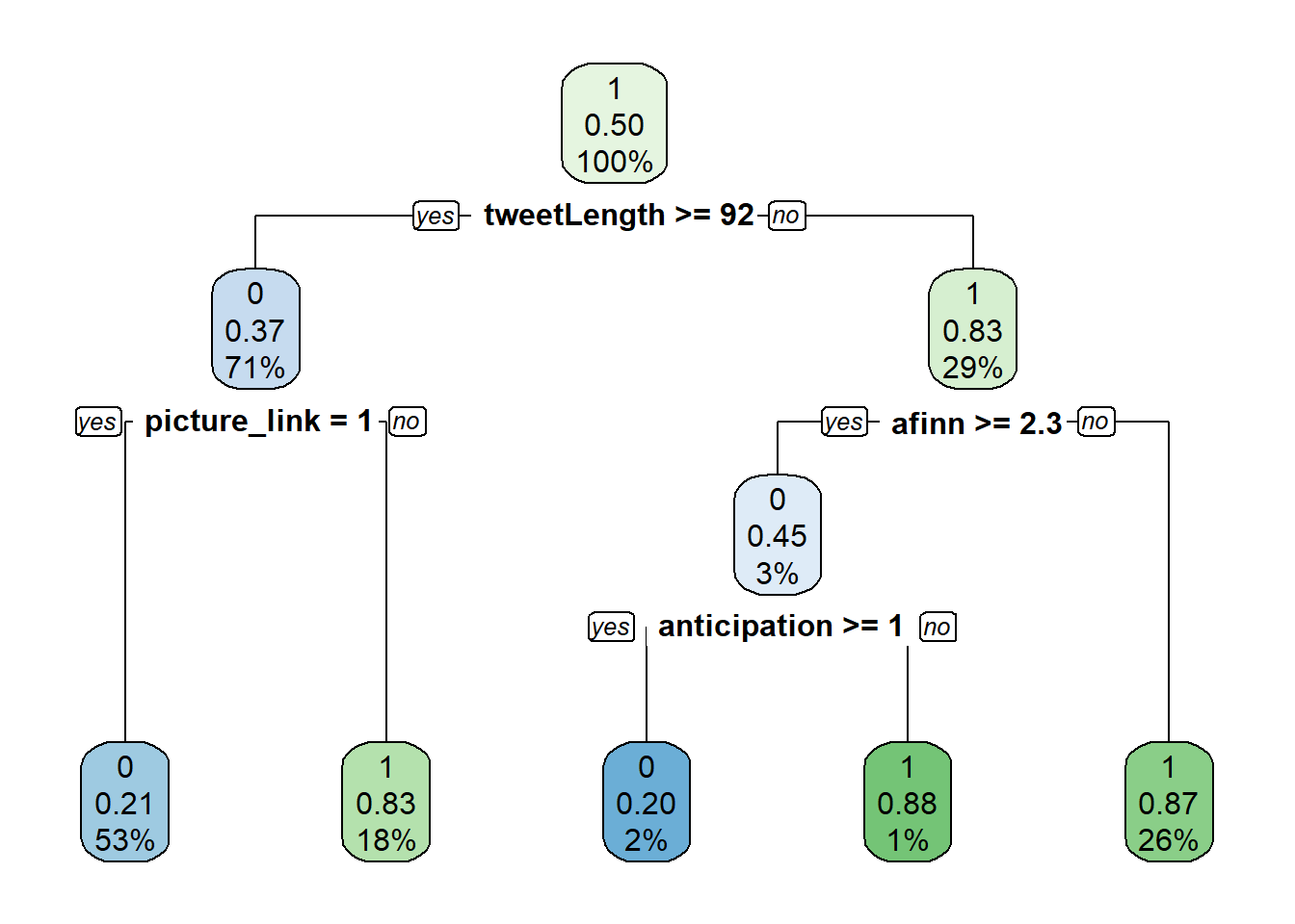
We produce additional models using the bagging, random forests, and gradient boosting methods.
set.seed(123)
bagging_model <- train(
  user ~ .,
  data = train,
  method = "treebag",
  trControl = trainControl(method = "oob"),
  keepX = T,
  nbagg = 100,
  importance = "impurity",
  control = rpart.control(minsplit = 2, cp = 0)
)
n_features <- length(setdiff(names(train), "user"))
rf_model <- ranger(
  user ~ .,
  data = train,
  mtry = floor(n_features * 0.5),
  respect.unordered.factors = "order",
  importance = "permutation",
  seed = 123
)
set.seed(123)  # for reproducibility
gbm_model <- gbm(
  formula = user ~ .,
  data = train,
  distribution = "gaussian",  # SSE loss function
  n.trees = 1000,
  shrinkage = 0.05,
  interaction.depth = 5,
  n.minobsinnode = 4,
  cv.folds = 10
)
We also display four variable importance plots to see which variables each model identified as significant.
vip(simple_model, num_features = 30) + ggtitle('Simple Decision Tree - Variable Importance Plot')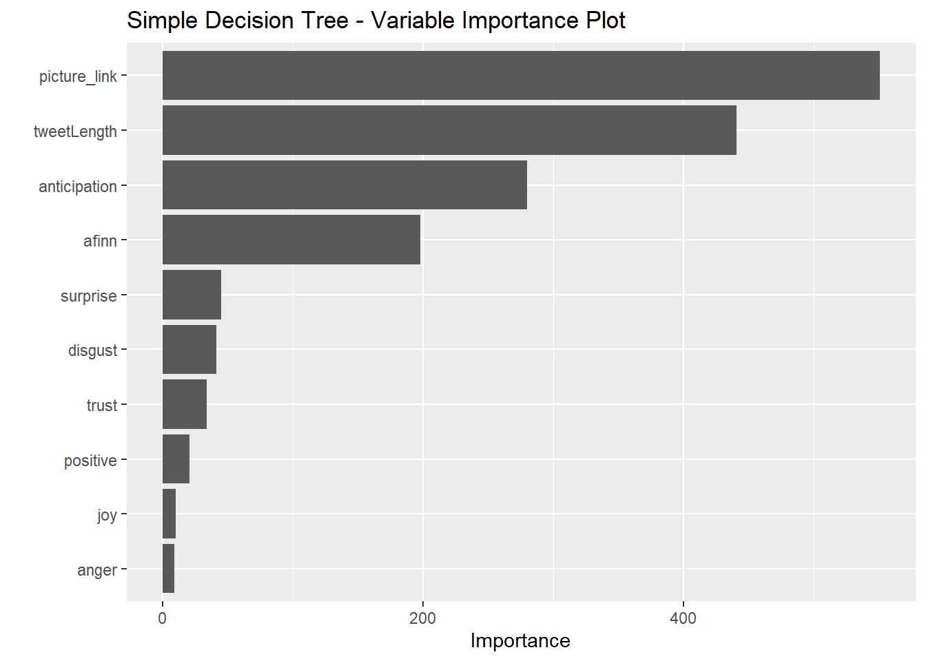
vip(bagging_model, num_features = 30) + ggtitle('Bagging - Variable Importance Plot')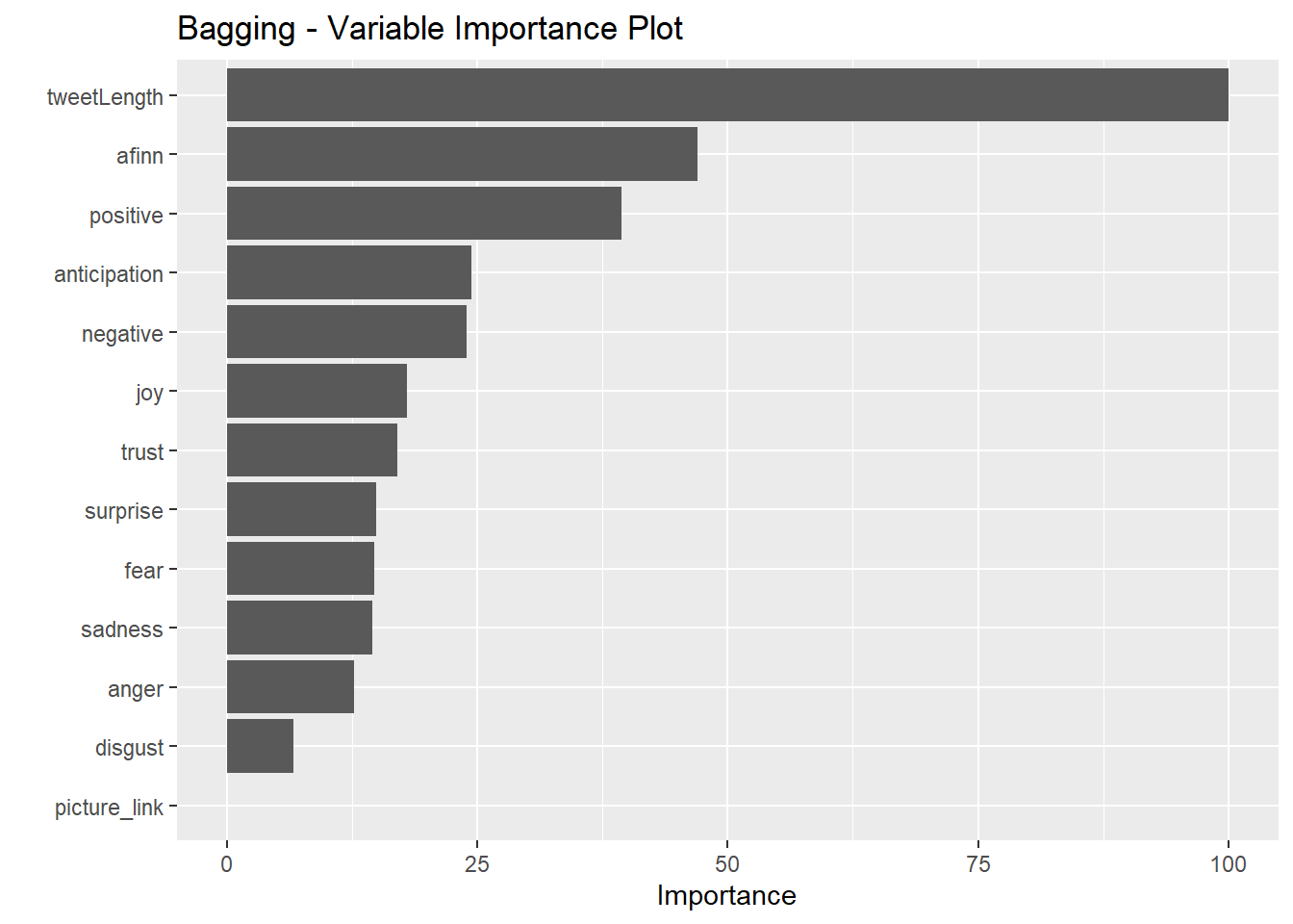
vip(rf_model, num_features = 30) + ggtitle('Random Forests - Variable Importance Plot')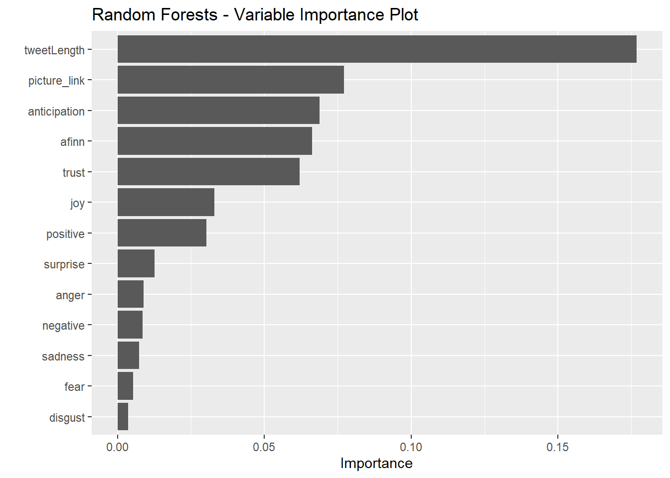
vip(gbm_model, num_features = 30) + ggtitle('Gradient Boosting - Variable Importance Plot')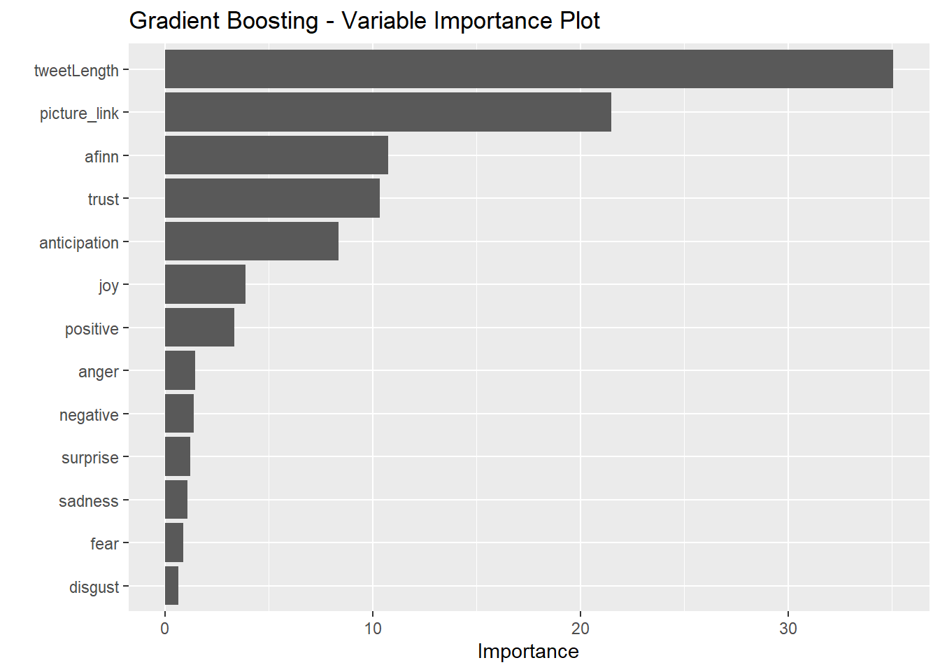
It seems that the simple decision tree placed the most importance on the presence of a picture/link. The bagging model, on the other hand places no importance on this variable. All four methods identified tweet length as strongly predictive of the user. All four heavily weighted anticipation sentiments and AFINN scores.
Results and Discussion
Now, we produce confusion matrices and show residual sum of squares for all tree-based methods—first evaluating their performance on the training set and then on the test set. Note again that a Tiktok tweet is encoded as 1, and a Facebook tweet is encoded as 0. The code is shown for the first matrix but not for subsequent ones for the sake of elegance.
Training Set Performance
Simple Decision Tree - Training Set:
## Confusion Matrix and Statistics
##
##           Reference
## Prediction    0    1
##          0 2215  583
##          1  332 1984
##
##                Accuracy : 0.8211
##                  95% CI : (0.8103, 0.8315)
##     No Information Rate : 0.502
##     P-Value [Acc > NIR] : < 2.2e-16
##
##                   Kappa : 0.6423
##
##  Mcnemar's Test P-Value : < 2.2e-16
##
##               Precision : 0.7916
##                  Recall : 0.8697
##                      F1 : 0.8288
##              Prevalence : 0.4980
##          Detection Rate : 0.4331
##    Detection Prevalence : 0.5471
##       Balanced Accuracy : 0.8213
##
##        'Positive' Class : 0
##
Bagging Method - Training Set:
## Confusion Matrix and Statistics
##
##           Reference
## Prediction    0    1
##          0 2458   57
##          1   89 2510
##
##                Accuracy : 0.9715
##                  95% CI : (0.9665, 0.9758)
##     No Information Rate : 0.502
##     P-Value [Acc > NIR] : <2e-16
##
##                   Kappa : 0.9429
##
##  Mcnemar's Test P-Value : 0.0103
##
##               Precision : 0.9773
##                  Recall : 0.9651
##                      F1 : 0.9712
##              Prevalence : 0.4980
##          Detection Rate : 0.4806
##    Detection Prevalence : 0.4918
##       Balanced Accuracy : 0.9714
##
##        'Positive' Class : 0
##
Random Forests Method - Training Set:
## Confusion Matrix and Statistics
##
##           Reference
## Prediction    0    1
##          0 2410   99
##          1  137 2468
##
##                Accuracy : 0.9539
##                  95% CI : (0.9477, 0.9594)
##     No Information Rate : 0.502
##     P-Value [Acc > NIR] : < 2e-16
##
##                   Kappa : 0.9077
##
##  Mcnemar's Test P-Value : 0.01602
##
##               Precision : 0.9605
##                  Recall : 0.9462
##                      F1 : 0.9533
##              Prevalence : 0.4980
##          Detection Rate : 0.4713
##    Detection Prevalence : 0.4906
##       Balanced Accuracy : 0.9538
##
##        'Positive' Class : 0
##
Gradient Boosting Method - Training Set:
## Using 806 trees...## Confusion Matrix and Statistics
##
## Reference
## Prediction 0 1
## 0 2297 303
## 1 250 2264
##
## Accuracy : 0.8919
## 95% CI : (0.883, 0.9002)
## No Information Rate : 0.502
## P-Value [Acc > NIR] : < 2e-16
##
## Kappa : 0.7837
##
## Mcnemar's Test P-Value : 0.02702
##
## Precision : 0.8835
## Recall : 0.9018
## F1 : 0.8926
## Prevalence : 0.4980
## Detection Rate : 0.4492
## Detection Prevalence : 0.5084
## Balanced Accuracy : 0.8919
##
## 'Positive' Class : 0
## Performance Summary and RSS
| type | total_errors | accuracy |
|---|---|---|
| Simple | 915 | 0.8210794 |
| Bagging | 146 | 0.9714509 |
| Random Forests | 236 | 0.9538522 |
| Gradient Boosting | 553 | 0.8918655 |
The rankings for accuracy on the training set are as follows: 1. Bagging method 2. Random forests 3. Gradient boosting method 4. Simple decision tree
We show the residual sum of squares for all four models on the training set below.
rss_simple_train <- sum((actual_train-simple_pred_train)^2)
rss_bagging_train <- sum((actual_train-bagging_pred_train)^2)
rss_rf_train <- sum((actual_train-rf_pred_train)^2)
rss_gb_train <- sum((actual_train-gb_pred_train)^2)
cat(paste0("Residual Sum of Squares on Training Set\n",
           "\nSimple model: ", rss_simple_train,
           "\nBagging model: ", rss_bagging_train,
           "\nRandom forests model: ", rss_rf_train,
           "\nGradient boosting model: ", rss_gb_train))
## Residual Sum of Squares on Training Set
##
## Simple model: 744.823130490417
## Bagging model: 148.955784690615
## Random forests model: 226.599946610086
## Gradient boosting model: 407.58762929458The bagging model performed the best on the training set, followed by the random forests method, the gradient boosting method, and the simple model in last place.
Now, we show confusion matrices for the test set.
Test Set Performance
Simple Decision Tree - Test Set:
actual_test <- test$user
simple_pred_test <-
  predict(simple_model, newdata = test) %>%
  as_tibble() %>%
  select(2) %>%
  unlist() %>%
  as.vector()
simple_test_confusion <-
  confusionMatrix(data = factor(round(simple_pred_test)),
                  reference = factor(actual_test), mode = "prec_recall")
simple_test_errors <-
  simple_test_confusion$table[2] +
  simple_test_confusion$table[3]
simple_test_accuracy <-
  as.numeric(simple_test_confusion$overall[1])
simple_test_confusion
## Confusion Matrix and Statistics
##
## Reference
## Prediction 0 1
## 0 562 138
## 1 89 489
##
## Accuracy : 0.8224
## 95% CI : (0.8003, 0.843)
## No Information Rate : 0.5094
## P-Value [Acc > NIR] : < 2.2e-16
##
## Kappa : 0.6441
##
## Mcnemar's Test P-Value : 0.001443
##
## Precision : 0.8029
## Recall : 0.8633
## F1 : 0.8320
## Prevalence : 0.5094
## Detection Rate : 0.4397
## Detection Prevalence : 0.5477
## Balanced Accuracy : 0.8216
##
## 'Positive' Class : 0
## Bagging Method - Test Set:
## Confusion Matrix and Statistics
##
##           Reference
## Prediction   0   1
##          0 550  92
##          1 101 535
##
##                Accuracy : 0.849
##                  95% CI : (0.8282, 0.8682)
##     No Information Rate : 0.5094
##     P-Value [Acc > NIR] : <2e-16
##
##                   Kappa : 0.6979
##
##  Mcnemar's Test P-Value : 0.5647
##
##               Precision : 0.8567
##                  Recall : 0.8449
##                      F1 : 0.8507
##              Prevalence : 0.5094
##          Detection Rate : 0.4304
##    Detection Prevalence : 0.5023
##       Balanced Accuracy : 0.8491
##
##        'Positive' Class : 0
##
Random Forests Method - Test Set:
## Confusion Matrix and Statistics
##
##           Reference
## Prediction   0   1
##          0 567  87
##          1  84 540
##
##                Accuracy : 0.8662
##                  95% CI : (0.8463, 0.8844)
##     No Information Rate : 0.5094
##     P-Value [Acc > NIR] : <2e-16
##
##                   Kappa : 0.7323
##
##  Mcnemar's Test P-Value : 0.8784
##
##               Precision : 0.8670
##                  Recall : 0.8710
##                      F1 : 0.8690
##              Prevalence : 0.5094
##          Detection Rate : 0.4437
##    Detection Prevalence : 0.5117
##       Balanced Accuracy : 0.8661
##
##        'Positive' Class : 0
##
Gradient Boosting Method - Test Set:
## Using 806 trees...## Confusion Matrix and Statistics
##
## Reference
## Prediction 0 1
## 0 568 93
## 1 83 534
##
## Accuracy : 0.8623
## 95% CI : (0.8422, 0.8807)
## No Information Rate : 0.5094
## P-Value [Acc > NIR] : <2e-16
##
## Kappa : 0.7244
##
## Mcnemar's Test P-Value : 0.4975
##
## Precision : 0.8593
## Recall : 0.8725
## F1 : 0.8659
## Prevalence : 0.5094
## Detection Rate : 0.4444
## Detection Prevalence : 0.5172
## Balanced Accuracy : 0.8621
##
## 'Positive' Class : 0
## Performance Summary and RSS
| type | total_errors | accuracy |
|---|---|---|
| Simple | 227 | 0.8223787 |
| Bagging | 193 | 0.8489828 |
| Random Forests | 171 | 0.8661972 |
| Gradient Boosting | 176 | 0.8622848 |
The rankings for accuracy on the test set are as follows:
- Random forests
- Gradient boosting method
- Bagging method
- Simple decision tree
Now, we show the residual sum of squares for each model with respect to the test set.
rss_simple_test <- sum((actual_test-simple_pred_test)^2)
rss_bagging_test <- sum((actual_test-bagging_pred_test)^2)
rss_rf_test <- sum((actual_test-rf_pred_test)^2)
rss_gb_test <- sum((actual_test-gb_pred_test)^2)
cat(paste0("Residual Sum of Squares on Test Set\n",
           "\nSimple model: ", rss_simple_test,
           "\nBagged model: ", rss_bagging_test,
           "\nRandom forests model: ", rss_rf_test,
           "\nGradient boost model: ", rss_gb_test))
## Residual Sum of Squares on Test Set
##
## Simple model: 185.903238689494
## Bagged model: 137.082023601223
## Random forests model: 120.747112472235
## Gradient boost model: 132.480675055803III. Results
Our sentiment analyses indicate that there are differences in sentiments of tweet communications between Tiktok and Facebook account. In general, while discussions surrounding Facebook uses more trust words, topics about TikTok uses more words that reflect anticipation. Tweets from Tiktok are more positive than those on Facebook. The random forests model performed the best on the test set even though it was only second best for the training set. However, that may be an indication that the bagging model was overfit to the training data, which caused it to perform worse on the test set than the random forests model.
When testing the models on our test data sets, for the simple model we observed 82.24% accuracy, for the bagging model we observed 84.9% accuracy, for the random forest we observed 86.62% accuracy, and for the gradient boosting model we observed 86.23% accuracy. Another good metric to compare is balanced accuracy, which is the average of specificity and sensitivity. For the simple model, balanced accuracy is 82.16%. For the bagging model, balanced accuracy is 84.91%. For the random forest, balanced accuracy is 86.61%. For the gradient boosting model, balanced accuracy is 86.21%.
In sum, it seems that the best model is the random forests model, with a test set accuracy score of 86.62%.
When analyzing the sum of squares difference between the actual tweeter and the predicted tweeter, the results were as follows:
Simple model: 744.823130490417
Bagging model: 148.955784690615
Random forests model: 226.599946610086
Gradient boosting model: 407.58762929458
IV. Conclusion
Looking at the analyses, it seems that the Facebook and TikTok accounts have systematically different Twitter presences. Facebook seems to respond more frequently to user fears, which are associated with words such as “secure” and “trust.” Whereas, TikTok focuses on generating excitement and offer prize giveaways, which is associated with “anticipation” words such as “winning” and “tomorrow.” Differences in tweet length also possibly reflect on the preferences of the target audience; TikTok users are younger and less likely to consume written information (it is a video platform, after all), and the opposite is true for Facebook. In sum, our predictive endeavor was successful, and we unveiled a number of useful insights from it.
V. Contributions
Ammar Plumber, Elaina Lin, Kim Nguyen, Meghan Aines, Ryan Karbowicz